POSTPROCESS DATA FILES |
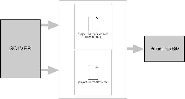
In the GiD postprocess you can study the results obtained from a solver program. The communication between the solver and the GiD Postprocess is made using files.
The solver program has to write the results in a file that must have the extension .post.res, or the old .flavia.res, and its name must be the project name.
The solver program can also (it is not mandatory) give to GiD the postprocess mesh, and should have the extension .post.msh, or the old .flavia.msh.
If this mesh is not provided by the solver program, GiD uses in the post-process, the preprocess mesh.
The extensions .msh and .res are also allowed, but
only the files with the extensions .post.res, or the old .flavia.res, and eventually .post.msh, or the old .flavia.msh,
will be automatically read by GiD when postprocessing the GiD project.
So, post-processing data files are ASCII files, and can be separated into two categories:
- Mesh Data File:
project_name.post.mshproject_name.flavia.mshfor volume and surface (3D or 2D) mesh information and - Results Data File:
project_name.post.resproject_name.flavia.resfor results information.
Note: ProjectName.post.msh, or the old ProjectName.flavia.msh, handles meshes of different
element types: points, lines, triangles, quadrilaterals, tetrahedras and hexahedras.
The old format, which only handles one type of element per file, is still supported inside GiD (see section Old postprocess mesh format).
If a project is loaded into GiD, when changing to PostProcess it will look
for ProjectName.post.res, or the old ProjectName.flavia.res. If a mesh information file
with name ProjectName.post.msh, or the old ProjectName.flavia.msh
is present, it will also be read, regardless of the information available from PreProcess.
- ProjectName.post.msh: (or the old ProjectName.flavia.msh)
The first file, which is named
ProjectName.flavia.msh, should contain nodal coordinates of the 3D, and its nodal connectivities and the material of each element. At the moment Only one set of nodal coordinates can be entered. Different kind of elements can be used but separated into different sets. If no material is supplied, GiD takes the material number equal to zero. - ProjectName.post.res: (or the old ProjectName.flavia.res) This second file must contain the nodal or gaussian variables. GiD allows the user to define as many nodal variables as desired, as well as several steps and analysis cases (limited only by the memory of the machine). Gauss points and results on these gauss points should also be in this file.
The files are created and read in the order that corresponds with the natural way of solving a finite element problem: mesh, surface definition and conditions and finally, evaluation of the results. The format of the read statements is normally free, i.e. it is necessary only to separate them by spaces.
Thus, the users can modify the files with any format, leaving spaces between each field and can also write out the results with as many decimals as desired. In case of error, the program warns the user about the type of mistake found.
GiD reads all the information directly from the pre-processing files in order to gain efficiency, whenever possible.
Postprocess mesh format: ProjectName.post.msh, ProjectName.flavia.msh |
Note: This postprocess mesh format needs GiD version 6.0 or higher.
Comments are allowed and should begin with a '#'.
Blank lines are also allowed.
To enter the mesh names and result names in another encoding, just write
# encoding your_encoding
for example:
# encoding utf-8
Inside this file one or more MESHes can be defined, each of them should:
- Begin with a header with this pattern:
MESH "mesh_name" dimension my_dimension Elemtype my_type Nnode my_number
beingMESH,dimension,elemtype,nnode: keywords that should be written as they are, case doesn't matter."mesh_name": an optional name for the mesh,my_dimension: 2 or 3 according to the geometric dimension of the mesh.my_type: one ofPoint,Linear,Triangle,Quadrilateral,Tetrahedra,HexahedraorPrism, describing the element type of thisMESH.my_number: the number of nodes ofmy_typeelement:Point: 1 node,Point connectivity: 
Linear: 2 or 3 nodes,Line connectivities: 

Triangle: 3 or 6 nodes,Triangle connectivities: 

Quadrilateral: 4, 8 or 9 nodes,Quadrilateral connectivities: 


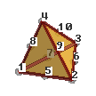
Tetrahedra: 4 or 10 nodes,Tetrahedral connectivities: 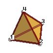
Hexahedra: 8, 20 or 27 nodes.Hexahedral connectivities: 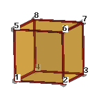
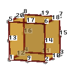
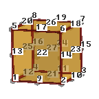
Prism: 6 or 15 nodes,Prism connectivities: 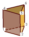
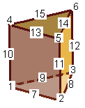
- an optional line describing its colour with
# color R G B, where R, G and B are the Red, Green and Blue components of the color written in integer format between 0 and 255, or in floating (real) format between 0.0 and 1.0. (Note that if 1 is found in the line it will be understood as integer, and so 1 above 255, rather than floating, and so 1 above 1.0)# color 127 127 0
In this way different colours can be specified for several meshes, taking into account that the# colorline must be between theMESHline and theCoordinatesline. - followed by the coordinates:
coordinates
   1   0.0   1.0   3.0
. . .

1000  -2.5   9.3  21.8
end coordinates
being- the pair
coordinatesandend coordinateskeywords that should be written as they are, case doesn't matter. - And between these keywords, the nodal coordinates of all the
MESHes or the current one.
Note: if eachMESHspecifies its own coordinates, the node number should be unique, for instance, ifMESH"mesh one" uses nodes 1..100, andMESH"other mesh" uses 50 nodes, they should be numbered up 100.
- the pair
- and followed by the elements connectivity
elements #el_num node_1 node_2 node_3 material 1 1 2 3 215 . . . 1000 32 48 23 215 end elementsbeing- the pair
elementsandend elementskeywords that should be written as they are, case doesn't matter. - And in-between the nodal connectivities for the
my_typeelements, Note: On elements of order higher than linear, the connectivities must written in hierarchical order, i.e. first the vertex nodes, then the middle ones. - and an optional material number.
- the pair
Mesh example |
This example clarifies this description:
#mesh of a table
MESH "board" dimension 3 ElemType Triangle  Nnode 3
# color 127 127 0
Coordinates
# node number   coordinate_x  coordinate_y  coordinate_z
    1             -5              3             -3
    2             -5              3              0
    3             -5              0              0
    4             -2              2              0
    5       -1.66667              3              0
    6             -5             -3             -3
    7             -2             -2              0
    8              0              0              0
    9             -5             -3              0
   10        1.66667              3              0
   11       -1.66667             -3              0
   12              2              2              0
   13              2             -2              0
   14        1.66667             -3              0
   15              5              3             -3
   16              5              3              0
   17              5              0              0
   18              5             -3             -3
   19              5             -3              0
end coordinates

#we put both material in the same MESH,
#but they could be separated into two MESH

Elements
# element  node_1   node_2  node_3 material_number
    5         19      17      13     3
    6          3       9       7     3
    7          2       3       4     3
    8         17      16      12     3
    9         12      16      10     3
   10         12      10       4     3
   11          7       9      11     3
   12          7      11      13     3
   13          2       4       5     3
   14          5       4      10     3
   15         19      13      14     3
   16         14      13      11     3
   17          3       7       4     3
   18         17      12      13     3
   19         13      12       8     4
   20         13       8       7     4
   21          7       8       4     4
   22          4       8      12     4
end elements

MESH    dimension 3 ElemType Linear  Nnode 2
Coordinates
#no coordinates then they are already in the first MESH
end coordinates

Elements
# element  node_1   node_2 material_number
    1          9       6     5
    2         19      18     5
    3         16      15     5
    4          2       1     5
end elements
Postprocess results format: ProjectName.post.res, ProjectName.flavia.res |
Note: The new postprocess results format needs GiD version 6.1.4b or higher.
Note: The code developers can download, from the GiD web page, the GiDpost tool, a C/C++/Fortran library to create postprocess files for GiD, in ASCII or compressed binary format.
This is the ASCII format description:
The first line of the files with results written in this new postprocess format should be:
GiD Post Results File 1.0
Comment lines are allowed and should begin with a '#'.
Blank lines are also allowed.
Results files can also be included with the keyword include, for instance:
include "My Other Results File"
This is useful, for instance, to share several GaussPoints definitions and ResultRangeTable
among different analysis.
This 'include' should be outside the Blocks of information.
There are several types of Blocks of information, all of them identified by a keyword:
GaussPointsInformation about gauss points: name, number of gauss points, natural coordinates, etc.ResultRangesTableInformation for the result visualization type Contour Ranges: name, ranges limits and ranges names.ResultInformation about a Result: name, analysis, analysis/time step, type of result, location, values.ResultGroupseveral results grouped in one block. These results share the same analysis, time step, and location ( nodes or gauss points).
Gauss Points |
To include Gauss points they must be defined before the Result which uses them.
Each Gauss points block are defined between a pair of GaussPoints and End GaussPoints.
The structure is as follows:
- Begin with a header with this pattern:
GaussPoints "gauss_points_name" Elemtype my_type "mesh_name"
beingGaussPoints,elemtype: keywords that should be written as they are, case doesn't matter."gauss_points_name": a name for thegauss pointsset, which will be used as reference by the results that are located on thesegauss points.my_type: one ofPoint,Linear,Triangle,Quadrilateral,TetrahedraorHexahedra, describing which element type are thesegauss pointsfor."mesh_name": an optional field. If this field is missing, thegauss pointsare defined for all the elements of typemy_type. If a mesh name is given, thegauss pointsare only defined for this mesh.
- followed by
gauss pointsproperties:Number of Gauss Points: number_gauss_points_per_element Nodes included Nodes not included Natural Coordinates: Internal Natural Coordinates: Given natural_coordinates_for_gauss_point_1 . . . natural_coordinates_for_gauss_point_n
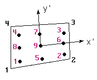
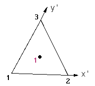
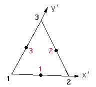
beingNumber of Gauss Points:number_gauss_points_per_element: a keyword that should be written as it is, case doesn't matter, followed by the number of gauss points per element that defines this set. IfNatural Coordinates:is set toInternal,number_gauss_points_per_elementshould be one of:- 1, 3, 6 for Triangles;
- 1, 4, 9 for Quadrilaterals;
- 1, 4, 10 for Tetrahedras;
- 1, 8, 27 for Hexahedras;
- 1, 6 for Prisms and
- 1, ... n points equally spaced over lines.
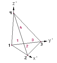
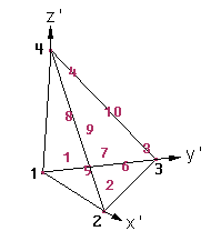
For tetrahedras the order of the Internal Gauss Points is this:
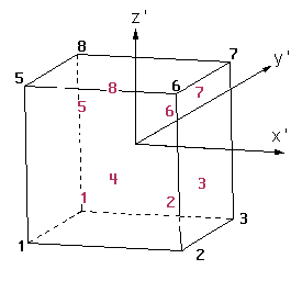
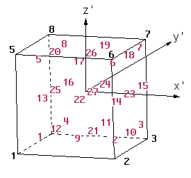
For hexahedras the order of the Internal Gauss Points is this:
For prisms the order of the Internal Gauss Points is this:
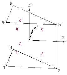
a=0.16666666, b=0.66666666
c=0.21132486, d=0.78867513
Internal coordinates:
( a, a, b) ( b, a, c) ( a, b, c)
( a, a, d) ( b, a, d) ( a, b, d)
Gauss Points in prisms Given natural coordinates for Gauss Points should range:
- between 0.0 and 1.0 for Triangles, Tetrahedras , Prisms, and
- between -1.0 and 1.0 for Quadrilaterals and Hexahedras.
number_gauss_points_per_elementnot included in the list written above.Nodes Included/Nodes not Included: keywords that should be written as they are, case doesn't matter, only necessary for gauss points onLinearelements which indicate whether the end nodes of theLinearelement are included in thenumber_gauss_points_per_elementcount or not.


Pseudo "gauss points" for lines with nodes included and not included Note: By now, Natural Coordinates for linear elements cannot be "
Given"Natural Coordinates: Internal/Natural Coordinates: Given: keywords that should be written as they are, case doesn't matter, telling if the natural coordinates are calculated internally by GiD, or are given in the following lines.
The natural coordinates should be written per line and gauss point.
- Ending with this tail:
End GaussPoints
beingEnd GaussPoints: a keyword that should be written as it is, case doesn't matter.
Here comes an example of results on Gauss Points:
GaussPoints "Board gauss internal" ElemType Triangle "board"
  Number Of Gauss Points: 3
  Natural Coordinates: internal
end gausspoints
Result Range Table |
To include a Result Range Table it must be defined before the Result which uses it.
Each Result Range Table is defined between a pair of ResultRangesTable and End ResultRangesTable.
The structure is as follows:
- Begin with a header with this pattern:
ResultRangesTable "ResultsRangeTableName"
beingResultRangesTable: a keyword which should be written as it is, case doesn't matter."ResultsRangeTableName": a name for theResult Ranges Table, which will be used as reference by the results that uses thisResult Ranges Table.
- followed by a list of
Ranges, each of them defined as follows:Min_Value - Max_Value: "Range Name"
beingMin_value: the minimum value of the range, may be void if theMax_valueis given. If void, the minimum value of the result will be used.Max_value: the maximum value of the range, may be void if theMin_valueis given. If void, the maximum value of the result will be used."Range Name": the name of the range which will appear on legends and labels.
- Ending with this tail:
End ResultRangesTable
beingEnd ResultRangesTable: a keyword that should be written as it is, case doesn't matter.
Several examples of results ranges table follows,
- Ranges defined for the whole result
ResultRangesTable "My table" # all the ranges are min <= res < max except # the last range is min <= res <= max - 0.3: "Less" 0.3 - 0.7: "Normal" 0.7 - : "Too much" End ResultRangesTable - Just a couple of ranges
ResultRangesTable "My table"
  0.3 - 0.7: "Normal"
  0.7 - 0.9: "Too much"
End ResultRangesTable
- or using the maximum of the result:
ResultRangesTable "My table"
  0.3 - 0.7: "Normal"
  0.7 -    : "Too much"
End ResultRangesTable
Result block |
Each Result block is identified by a Result header, followed by several
optional properties: component names, ranges table, and the result values, defined the
pair of Values and End Values.
The structure is as follows:
- Begin with a header with this pattern:
Result "result name" "analysis name" step_value my_result_type my_location "location name"
beingResult: a keyword that should be written as it is, case doesn't matter."result name": a name for theResult, which will be used for menus."analysis name": the name of the analysis of thisResult, which will be used for menus.step_value: the value of the step inside the analysis"analysis name".my_type: type of theResult, should be one ofScalar,Vector,Matrix,PlainDeformationMatrix,MainMatrix,LocalAxes.my_location: where is theResultlocated, should be one ofOnNodes,OnGaussPoints. If theResultisOnGaussPointsa"location name"should be entered."location name": name of theGauss Pointson which theResultis defined.
- followed by optional
resultproperties:ResultRangesTable "Name of a result ranges table" ComponentNames "Name of Component 1", "Name of Component 2"
beingResultRangesTable"Name of a result ranges table": ( optional) a keyword that should be written as it is, case doesn't matter, followed by the name of the previously definedTesult Ranges Tablewhich will be used if theContour Rangesresult visualization is chosen ( see section Result Range Table).ComponentNames"Name of Component 1", "Name of Component 2": ( optional) a keyword that should be written as it is, case doesn't matter, followed by the names of the components of the results which will be used in GiD. The number ofComponent Namesare these:- One for a
Scalar Result - Three for a
Vector Result - Six for a
Matrix Result - Four for a
PlainDeformationMatrix Result - Six for a
MainMatrix Result - Three for a
LocalAxes Result
- One for a
- and ending with the
resultvalues:Values node_or_elem_number component_1_value component_2_value . . . node_or_elem_number component_1_value component_2_value End Values
beingValues: a keyword that should be written as it is, case doesn't matter, which indicates the beginning of theresult's valuessection.- The lines
node_or_elem_number component_1_value component_2_value. . .node_or_elem_number component_1_value component_2_value
- if the
Resultis locatedOnNodes: the number of nodes defined inProjectName.flavia.msh - if the
Resultis locatedOnGaussPoints "My GP": if theGauss Points "My GP"are defined for the mesh"My mesh", the limit is the number of gauss points in"My GP"multiplied by the number of elements of the mesh"My mesh".
For results in gauss points, each element must have 'ngauss' lines of results.for example, if the number of gauss points is 3 , then must appear 3 lines of gauss point result for a element Values 1 1.155 2.9 3.955 End Values
Holes are allowed in any result. The nodes, elements, with no result defined will not be drawn, i.e. they will appear transparent.
The number of components for eachResult Valueare:- for
Scalarresults: one component
result_number_i scalar_value - for
Vectorresults: three components, with an optional fourth component for signed modules
result_number_i x_value y_value z_value
result_number_i x_value y_value z_value signed_module_value - for
Matrixresults: three components ( 2D models) or six components (3D models)
2D:result_number_i Sxx_value Syy_value Sxy_value
3D:result_number_i Sxx_value Syy_value Szz_value Sxy_value Syz_value Sxz_value - for
PlainDeformationMatrixresults: four components
result_number_i Sxx_value Syy_value Sxy_value Szz_value - for
MainMatrixresults: twelve components
result_number_i Si_value Sii_value Siii_value Vix_value Viy_value Viz_value Viix_value Viiy_value Viiz_value Viiix_value Viiiy_value Viiiz_value - for
LocalAxesresults: three components describing the Euler angles
result_number_i euler_ang_1_value euler_ang_2_value euler_ang_3_value
End Values: a keyword that should be written as it is, case doesn't matter., which indicates the end of theresult's valuessection.
Note: for Matrix and PlainDeformationMatrix results, the
Si, Sii and Siii components are calculated by GiD, which represents the eigen values & vectors
of the matrix results, and which are ordered according to the eigen value.
Result group |
Results canbe grouped into on block. These results belongs to the same time step of the same analysis and are located in the same place. So all the results in the group are nodal results or are defined over the same gauss points set.
Each Result group is identified by a ResultGroup header, followed by
the results descriptions and its optional properties, such as components names
and ranges tables, and the results values, between the pair Values
... End values.
The structure is as follows:
- Begin with a header with this pattern
ResultGroup "analysis name" step_value my_location "location name"
beingResultGroup: a keyword that should be written as it is, case doesn't matter."analysis name": the name of the analysis of thisResultGroup, which will be used for menus.step_value: the value of the step inside the analysis"analysis name".my_location: where is theResultGrouplocated, should be one ofOnNodes,OnGaussPoints. If theResultGroupisOnGaussPointsa"location name"should be entered."location name": name of theGauss Pointson which theResultGroupis defined.
- followed by, at least one, the results descriptions of the group:
ResultDescription "result name" my_result_type[:components_number]
  ResultRangesTable "Name of a result ranges table"
  ComponentNames "Name of Component 1", "Name of Component 2"
beingResultDescription: a keyword that should be written as it is, case doesn't matter."result name": a name for theResult, which will be used for menus.my_type: type of theResult, should be one ofScalar,Vector,Matrix,PlainDeformationMatrix,MainMatrix,LocalAxes. The number of components for each type is as follows:- One for a
Scalar: the_scalar_value - Three for a
Vector: X, Y and Z - Six for a
Matrix: Sxx, Syy, Szz, Sxy, Syz and Sxz - Four for a
PlainDeformationMatrix: Sxx_value, Syy, Sxy and Szz - Twelve for a
MainMatrix: Si, Sii, Siii, ViX, ViY, ViZ, ViiX, ViiY, ViiZ, ViiiX, ViiiY and ViiiZ - Three for a
LocalAxes: euler_ang_1, euler_ang_2 and euler_ang_3
Vector:2,Vector:3orVector:4: which specify:Vector:2: X and YVector:3: X, Y and Z #itemVector:4: X, Y, Z and |Vector| (module of the vector, with sign)
Vector) is 3 components per vector.Matrix:3orMatrix:6: which specify:Matrix:3: Sxx, Syy and SxyMatrix:6: Sxx, Syy, Szz, Sxy, Syz and Sxz
Matrix) is 6 components for matrices.
ResultDescription "Displacements" Vector:2
ResultDescription "2D matrix" Matrix:3
ResultDescription "LineDiagramVector" Vector:4
- One for a
ResultRangesTable"Name of a result ranges table": ( optional) a keyword that should be written as it is, case doesn't matter, followed by the name of the previously definedTesult Ranges Tablewhich will be used if theContour Rangesresult visualization is chosen ( see section Result Range Table).ComponentNames"Name of Component 1", "Name of Component 2": ( optional) a keyword that should be written as it is, case doesn't matter, followed by the names of the components of the results which will be used in GiD. The number ofComponent Namesare these:- One for a
Scalar Result - Three for a
Vector Result - Six for a
Matrix Result - Four for a
PlainDeformationMatrix Result - Six for a
MainMatrix Result - Three for a
LocalAxes Result
- One for a
- and ending with the results values:
Values
 location_1 result_1_component_1_value result_1_component_2_value result_1_component_3_value result_2_component_2_value result_2_component_2_value result_2_component_3_value
 . . .

 location_n result_1_component_1_value result_1_component_2_value result_1_component_3_value result_2_component_2_value result_2_component_2_value result_2_component_3_value
End Values
beingValues: a keyword that should be written as it is, case doesn't matter, which indicates the beginning of theresult's valuessection.- The lines
location_1 result_1_component_1_value result_1_component_2_value result_1_component_3_value result_2_component_2_value result_2_component_2_value result_2_component_3_value. . .location_n result_1_component_1_value result_1_component_2_value result_1_component_3_value result_2_component_2_value result_2_component_2_value result_2_component_3_value
ResultDescriptionfor each location. All the results values for the location 'i' should be written in the same line 'i'.
The number of results values are limited to:- if the
Resultis locatedOnNodes: the number of nodes defined inProjectName.post.msh, or the oldProjectName.flavia.msh. - if the
Resultis locatedOnGaussPoints "My GP": if theGauss Points "My GP"are defined for the mesh"My mesh", the limit is the number of gauss points in"My GP"multiplied by the number of elements of the mesh"My mesh".
The number of components for eachResultDescriptionare:- for
Scalarresults: one component
result_number_i scalar_value - for
Vectorresults: three components
result_number_i x_value y_value z_value - for
Matrixresults: six components (3D models)
3D:result_number_i Sxx_value Syy_value Szz_value Sxy_value Syz_value Sxz_value - for
PlainDeformationMatrixresults: four components
result_number_i Sxx_value Syy_value Sxy_value Szz_value - for
MainMatrixresults: twelve components
result_number_i Si_value Sii_value Siii_value Vix_value Viy_value Viz_value Viix_value Viiy_value Viiz_value Viiix_value Viiiy_value Viiiz_value - for
LocalAxesresults: three components describing the Euler angles
result_number_i euler_ang_1_value euler_ang_2_value euler_ang_3_value
End Values: a keyword that should be written as it is, case doesn't matter., which indicates the end of theresult's group valuessection.
Note: Vectors in a ResultGroup have always three components.
Note: Matrix in a ResultGroup have always six components.
Note: all the result of one node or gauss point, should be written in the same line.
Note: for Matrix and PlainDeformationMatrix results, the
Si, Sii and Siii components are calculated by GiD, which represents the eigen values & vectors
of the matrix results, and which are ordered according to the eigen value.
Nodal ResultGroup example:
ResultGroup "Load Analysis" 1 OnNodes
  ResultDescription "Ranges test" Scalar
    ResultRangesTable "My table"
  ResultDescription "Scalar test" Scalar
    ResultRangesTable "Pressure"
  ResultDescription "Displacements" Vector
    ComponentNames "X-Displ", "Y-Displ" "Z-Displ"
  ResultDescription "Nodal Stresses" Matrix
    ComponentNames "Sx", "Sy", "Sz", "Sxy", "Syz", "Sxz"
Values
    1 0.0           0.00000E+00 0.00000E+00  0.00000E+00 0.0 0.55014E+00  0.97276E-01 -0.15427E+00 0.0 0.0 0.0
    2 6.4832835e-01 0.20855E-04 0.20855E-04 -0.19174E-04 0.0 0.50676E+00  0.33886E-01 -0.10559E+00 0.0 0.0 0.0
    3 0.0           0.35517E-04 0.35517E-04 -0.37637E-04 0.0 0.37765E+00  0.44121E-02 -0.54703E-01 0.0 0.0 0.0
...

  115 7.8873599e-01 0.42781E-04 0.42781E-04 -0.17594E-03 0.0 0.15692E-01 -0.15847E-01 -0.30077E-01 0.0 0.0 0.0
  116 7.4978158e-01 0.24357E-04 0.24357E-04 -0.18974E-03 0.0 0.21668E-02 -0.96841E-02 -0.23115E-01 0.0 0.0 0.0
End Values
Gauss Points ResultGroup example:
GaussPoints "My Gauss" ElemType Triangle "2D Beam"
  Number Of Gauss Points: 3
  Natural Coordinates: Internal
End gausspoints

ResultGroup "Load Analysis" 1 OnGaussPoints "My Gauss"
  ResultDescription "Gauss test"  Scalar
  ResultDescription "Vector Gauss" Vector
  ResultDescription "Gauss Points Stresses" PlainDeformationMatrix
Values
  1 1.05   1 0                      0.0     -19.4607 -1.15932 -1.43171 -6.18601
    2.1	   0 1                      0.0     -19.4607 -1.15932 -1.43171 -6.18601
    3.15   1 1                      0.0     -19.4607 -1.15932 -1.43171 -6.18601
  2 1.2	   0 0                      0.0     -20.6207 0.596461 5.04752 -6.00727
    2.25   0 0                      0.0     -20.6207 0.596461 5.04752 -6.00727
    3.3	   2.0855e-05 -1.9174e-05   0.0     -20.6207 0.596461 5.04752 -6.00727
  3 1.35   2.0855e-05 -1.9174e-05   0.0     -16.0982 -1.25991 2.15101 -5.20742
    2.4	   2.0855e-05 -1.9174e-05   0.0     -16.0982 -1.25991 2.15101 -5.20742
    3.45   2.0855e-05 -1.9174e-05   0.0     -16.0982 -1.25991 2.15101 -5.20742
...

191 29.55  4.2781e-05 -0.00017594   0.0     -0.468376 12.1979 0.610867 3.51885
    30.6   4.2781e-05 -0.00017594   0.0     -0.468376 12.1979 0.610867 3.51885
    31.65  4.2781e-05 -0.00017594   0.0     -0.468376 12.1979 0.610867 3.51885
192 29.7   4.2781e-05 -0.00017594   0.0     0.747727 11.0624 1.13201 3.54303
    30.75  4.2781e-05 -0.00017594   0.0     0.747727 11.0624 1.13201 3.54303
    31.8   2.4357e-05 -0.00018974   0.0     0.747727 11.0624 1.13201 3.54303
End Values
Results example |
Here comes an example of results for the table of the previous example (see section Mesh example):
GiD Post Results File 1.0

GaussPoints "Board gauss internal" ElemType Triangle "board"
  Number Of Gauss Points: 3
  Natural Coordinates: internal
end gausspoints

GaussPoints "Board gauss given" ElemType Triangle "board"
  Number Of Gauss Points: 3
  Natural Coordinates: Given
      0.2 0.2
      0.6 0.2
      0.2 0.6
End gausspoints

GaussPoints "Board elements" ElemType Triangle "board"
  Number Of Gauss Points: 1
  Natural Coordinates: internal
end gausspoints

GaussPoints "Legs gauss points" ElemType Linear
  Number Of Gauss Points: 5
  Nodes included
  Natural Coordinates: Internal
End Gausspoints

ResultRangesTable "My table"
# el ultimo rango es min <= res <= max
      - 0.3: "Less"
  0.3 - 0.9: "Normal"
  0.9 - 1.2: "Too much"
End ResultRangesTable

Result "Gauss element" "Load Analysis" 1 Scalar OnGaussPoints "Board elements"
Values
    5     0.00000E+00
    6     0.20855E-04
    7     0.35517E-04
    8     0.46098E-04
    9     0.54377E-04
   10     0.60728E-04
   11     0.65328E-04
   12     0.68332E-04
   13     0.69931E-04
   14     0.70425E-04
   15     0.70452E-04
   16     0.51224E-04
   17     0.32917E-04
   18     0.15190E-04
   19    -0.32415E-05
   20    -0.22903E-04
   21    -0.22919E-04
   22    -0.22283E-04
End Values

Result "Displacements" "Load Analysis"  1  Vector OnNodes
ResultRangesTable "My table"
ComponentNames "X-Displ", "Y-Displ", "Z-Displ"
Values
    1    0.0   0.0   0.0
    2   -0.1   0.1   0.5
    3    0.0   0.0   0.8
    4   -0.04  0.04  1.0
    5   -0.05  0.05  0.7
    6    0.0   0.0   0.0
    7   -0.04 -0.04  1.0
    8    0.0   0.0   1.2
    9   -0.1  -0.1   0.5
   10    0.05  0.05  0.7
   11   -0.05 -0.05  0.7
   12    0.04  0.04  1.0
   13    0.04 -0.04  1.0
   14    0.05 -0.05  0.7
   15    0.0   0.0   0.0
   16    0.1   0.1   0.5
   17    0.0   0.0   0.8
   18    0.0   0.0   0.0
   19    0.1  -0.1   0.5
End Values

Result "Gauss displacements" "Load Analysis" 1 Vector OnGaussPoints "Board gauss given"
Values
    5    0.1  -0.1   0.5
         0.0   0.0   0.8
         0.04 -0.04  1.0
    6    0.0   0.0   0.8
        -0.1  -0.1   0.5
        -0.04 -0.04  1.0
    7   -0.1   0.1   0.5
         0.0   0.0   0.8
        -0.04  0.04  1.0
    8    0.0   0.0   0.8
         0.1   0.1   0.5
         0.04  0.04  1.0
    9    0.04  0.04  1.0
         0.1   0.1   0.5
         0.05  0.05  0.7
   10    0.04  0.04  1.0
         0.05  0.05  0.7
        -0.04  0.04  1.0
   11   -0.04 -0.04  1.0
        -0.1  -0.1   0.5
        -0.05 -0.05  0.7
   12   -0.04 -0.04  1.0
        -0.05 -0.05  0.7
         0.04 -0.04  1.0
   13   -0.1   0.1   0.5
        -0.04  0.04  1.0
        -0.05  0.05  0.7
   14   -0.05  0.05  0.7
        -0.04  0.04  1.0
         0.05  0.05  0.7
   15    0.1  -0.1   0.5
         0.04 -0.04  1.0
         0.05 -0.05  0.7
   16    0.05 -0.05  0.7
         0.04 -0.04  1.0
        -0.05 -0.05  0.7
   17    0.0   0.0   0.8
        -0.04 -0.04  1.0
        -0.04  0.04  1.0
   18    0.0   0.0   0.8
         0.04  0.04  1.0
         0.04 -0.04  1.0
   19    0.04 -0.04  1.0
         0.04  0.04  1.0
         0.0   0.0   1.2
   20    0.04 -0.04  1.0
         0.0   0.0   1.2
        -0.04 -0.04  1.0
   21   -0.04 -0.04  1.0
         0.0   0.0   1.2
        -0.04  0.04  1.0
   22   -0.04  0.04  1.0
         0.0   0.0   1.2
         0.04  0.04  1.0
End Values

Result "Legs gauss displacements" "Load Analysis" 1 Vector OnGaussPoints "Legs gauss points"
Values
    1   -0.1  -0.1   0.5
        -0.2  -0.2   0.375
        -0.05 -0.05  0.25
         0.2   0.2   0.125
         0.0   0.0   0.0
    2    0.1  -0.1   0.5
         0.2  -0.2   0.375
         0.05 -0.05  0.25
        -0.2   0.2   0.125
         0.0   0.0   0.0
    3    0.1   0.1   0.5
         0.2   0.2   0.375
         0.05  0.05  0.25
        -0.2  -0.2   0.125
         0.0   0.0   0.0
    4   -0.1   0.1   0.5
        -0.2   0.2   0.375
        -0.05  0.05  0.25
         0.2  -0.2   0.125
         0.0   0.0   0.0
End Values
Re-meshing and adaptivity |
If the same meshes are used for all the analysis the following section can be skipped.
A new concept has been introduced in Postprocess: Group to allow the postprocess
of problems which require re-meshing or adaptive meshes.
Meshes which belongs to a group should be defined between the pair
Group "group name"
MESH "mesh_name" dimension ...
...
end elements

MESH "another_mesh" ...
...
end elements
end group
Results which are referred to one of the groups should be written between the pair
OnGroup "group name"
Result "result name"
...
end values
...
end ongroup
Note: As of GiD version 7.7.3b only one group is allowed at a time, i.e., one group can be defined across several steps of the analysis and only one. Care should be taken so that groups do not overlap inside the same step/analysis.
For instance, an analysis which is 10 steps long:
- steps 1, 2, 3 and 4 uses: an 'environment' mesh of 10000 elements and a 'body'
mesh of 10000 elements
   MESH "environment" ...
   Coordinates
   ...
   10000 ...
   end elements
   MESH "body" ...
   ...
   20000 ...
   end elements
and its resultsGiD Post Results File 1.0 ... Results "result 1" "time" 1.0 ... ... Results "result 1" "time" 2.0 ... ... Results "result 1" "time" 3.0 ... ... Results "result 1" "time" 4.0 ... ... end values
- steps 5, 6, 7 and 8 uses: now, with some refinement, the 'environment' mesh now
has 15000 elements and the 'body' mesh needs 20000 elements
   MESH "environment" ...
   Coordinates
   ...
   15000 ...
   end elements
   MESH "body" ...
   ...
   35000 ...
   end elements
and its resultsGiD Post Results File 1.0 ... Results "result 1" "time" 5.0 ... ... Results "result 1" "time" 6.0 ... ... Results "result 1" "time" 7.0 ... ... Results "result 1" "time" 8.0 ... ... end values
- steps 9 and 10: the last meshes are 20000 and 40000 elements big, respectively
   MESH "environment" ...
   Coordinates
   ...
   20000 ...
   end elements
   MESH "body" ...
   ...
   60000 ...
   end elements
and its resultsGiD Post Results File 1.0 ... Results "result 1" "time" 9.0 ... ... Results "result 1" "time" 10.0 ... ... end values
There are two ways to postprocess this:
- store the information in three pairs (or three binary files)
- steps_1_2_3_4.post.msh and steps_1_2_3_4.post.msh ( or steps_1_2_3_4.post.bin)
- steps_5_6_7_8.post.msh and steps_5_6_7_8.post.msh ( or steps_5_6_7_8.post.bin)
- steps_9_10.post.msh and steps_9_10.post.msh ( or steps_9_10.post.bin)
Open multiple' option (see section Files menu) to selected the six files (or three); or - write them in only two files (one in binary) by using the Group concept:
- all_analysis.post.msh (note the
group - end grouppairs)Group "steps 1, 2, 3 and 4" MESH "environment" ... ... MESH "body" ... ... end group Group "steps 5, 6, 7 and 8" MESH "environment" ... ... MESH "body" ... ... end group Group "steps 9 and 10" MESH "environment" ... ... MESH "body" ... ... end group
and - all_analysis.post.res (note the
ongroup - end ongrouppairs)GiD Post Results File 1.0 OnGroup "steps 1, 2, 3 and 4" ... Results "result 1" "time" 1.0 ... ... Results "result 1" "time" 2.0 ... ... Results "result 1" "time" 3.0 ... ... Results "result 1" "time" 4.0 ... ... end ongroup OnGroup "steps 5, 6, 7 and 8" ... Results "result 1" "time" 5.0 ... ... Results "result 1" "time" 6.0 ... ... Results "result 1" "time" 7.0 ... ... Results "result 1" "time" 8.0 ... ... end ongroup OnGroup "steps 9 and 10" ... Results "result 1" "time" 9.0 ... ... Results "result 1" "time" 10.0 ... ... end ongroup
Openoption. - all_analysis.post.msh (note the
Old postprocess results format |
This file is a complete list of the dumped results, where each result will be organized as follows:
Set 1: Header. Results description
The total number of lines in this set is 1, composed by 1 character string, 1 integer, 1 real, 1 optional character string what depends on the first integer, plus 3 integers:
descr_menu load_type step_val [load_desc]
data_type data_loc desc_comp ["gauss_points_name"]
where:
descr_menu= results title that will appear on the menus (maximum 15 characters without any blank spaces inside).load_type= type of analysis effectuated to obtain this result:- 1 - time analysis (Time Step).
- 2 - load analysis (Load Step).
- 3 - frequency analysis (Frequency).
- 4 - user defined analysis (User Step).
step_val= number of steps inside the analysis.load_desc= description, without any blank spaces inside, of the analysis that will appear on the menus. This field must only be specified when the analysis is defined by the user (load_type= 4).data_type= kind of results:- 1 - scalar.
- 2 - vector.
- 3 - matrix.
- 4 - 2D plane deformation matrix
- 5 - Main stresses ( 3 modules and 3 vectors)
- 6 - Euler angles ( for local axes)
data_loc= position of the data: 1 - on the nodes. 2 - on the Gauss points.desc_comp= specification of the existence of a description of each component that will be displayed as a menu's button:- 0 - no description (inside GiD, the program itself creates the description for the corresponding components).
- 1 - there will be a description, without any blank spaces inside, of the components, with one component per line.
"gauss_points_name": optional field that specifies the set of gauss points to be used (new gauss point format see section Gauss Points). If not specified the general gauss points definition will be used (old format).
Set 2: Description of the components
The description of each one of the result's components, without any blank spaces inside, should be described here if needed, one per line. The number of lines will be as follows:
- One line if it is a scalar.
- Three lines if it is vector.
- Six lines if it is a matrix.
- Four lines if it is a 2D plane deformation matrix.
- Six lines if it is Main Stresses.
- Three lines if it is a Euler angles result.
This description will appear in different menus to select the variable to be displayed at each stage.
Note: GiD also supports 2D results types, so description components can be two for vectors, and three or four for matrix and plane strain analysis, respectively.
Set 3: Results
The total number of lines in this set is the total number of points if data_loc =
1 or the total number of elements multiplied by the number of Gauss points per element
if data_loc = 2. The definition of the results is itemized below.
- Scalar: Each line is composed by one integer plus one real number:
i result[i]
- where:
i= node or Gauss point number.result[i]= value of the result on the node or Gauss point numberi.
- Vector: Each line is composed by 1 integer plus 3 reals:
i result_x[i] result_y[i] result_z[i] result_m[i]
- where:
i= node or Gauss point number.result_x[i]= value of the x_component of the result on the node or Gauss point numberi.result_y[i]= value of the y_component of the result on the node or Gauss point numberi.result_z[i]= value of the x_component of the result on the node or Gauss point numberi. Optional if a 2D result type is specified. Should be specified ifresult_m[i]is given.result_m[i]= value of the signed module of the vector (to allow negative values for the vector diagram result view). This component is optional, if not specified, GiD calculates the module of the entered vector. But if it is defined,result_z[i]should be defined too.
- Matrix: Each line is composed by 1 integer plus 6 reals:
i result_Sxx[i] result_Syy[i] result_Szz[i]
result_Sxy[i] result_Syz[i] result_Sxz[i]
- where:
i= node or Gauss point number.result_Sxx[i]= value of the xx_component of the result on the node or Gauss point numberi.result_Syy[i]= value of the yy_component of the result on the node or Gauss point numberi.result_Szz[i]= value of the zz_component of the result on the node or Gauss point numberi. Optional if a 2D result type is specified that is not a plane deformation matrix.result_Sxy[i]= value of the xy_component of the result on the node or Gauss point numberi.result_Syz[i]= value of the yz_component of the result on the node or Gauss point numberi. Optional if a 2D result type is specified.result_Sxz[i]= value of the xz_component of the result on the node or Gauss point numberi. Optional if a 2D result type is specified.
- Main Stresses: Another way to give Stresses to GiD is entering modules and vectors of these main stresses, so each line is composed by 1 integer plus 12 reals:
i result_Si[i] result_Sii[i] result_Siii[i]
result_Vi_x[i] result_Vi_y[i] result_Vi_z[i]
result_Vii_x[i] result_Vii_y[i] result_Vii_z[i]
result_Viii_x[i] result_Viii_y[i] result_Viii_z[i]
- where:
i= node or Gauss point number.result_Si[i]= value of the Si_module of the result on the node or Gauss point numberi.result_Sii[i]= value of the Sii_module of the result on the node or Gauss point numberi.result_Siii[i]= value of the Siii_module of the result on the node or Gauss point numberi. Optional if a 2D result type is specified.result_Vi_x[i]= value of the X_component of the vector Si on the node or Gauss point numberi.result_Vi_y[i]= value of the Y_component of the vector Si on the node or Gauss point numberi.result_Vi_z[i]= value of the Z_component of the vector Si on the node or Gauss point numberi. Optional if a 2D result type is specified.result_Vii_x[i]= value of the X_component of the vector Sii on the node or Gauss point numberi.result_Vii_y[i]= value of the Y_component of the vector Sii on the node or Gauss point numberi.result_Vii_z[i]= value of the Z_component of the vector Sii on the node or Gauss point numberi. Optional if a 2D result type is specified.result_Viii_x[i]= value of the X_component of the vector Siii on the node or Gauss point numberi.result_Viii_y[i]= value of the Y_component of the vector Siii on the node or Gauss point numberi.result_Viii_z[i]= value of the Z_component of the vector Siii on the node or Gauss point numberi. Optional if a 2D result type is specified.
- Local Axes: Local Axes are entered using the Euler angles that define them, so each line is composed by 1 integer plus 3 reals:
i euler_ang_1[i] euler_ang_2[i] euler_ang_3[i]
- where:
i= node or Gauss point number.euler_ang_1[i]= value of the 1st. angle of Euler of the local axis on the node or Gauss point numberi.euler_ang_2[i]= value of the 2nd. angle of Euler of the local axis on the node or Gauss point numberi.euler_ang_3[i]= value of the 3rd. angle of Euler of the local axis on the node or Gauss point numberi.
Note: for Matrix and PlainDeformationMatrix results, the
Si, Sii and Siii components are calculated by GiD, which represents the eigen values & vectors
of the matrix results, and which are ordered according to the eigen value.
Results on GaussPoints: When defining results on Gauss Points using the new Gauss points
format, i.e. giving a "gauss_points_name" on the Result's Header description, the
results should be given on a per element basis specifying the element number only once. For instance:
assuming a three gauss points set named "GaussTriang" has been defined over triangles, there are only two triangles, then a supposed 'Displacement' result will look like this:
GaussDISPLAC.   2    1    2    2    0 "GaussTriang"
    5    0.1  -0.1   0.5
         0.0   0.0   0.8
         0.04 -0.04  1.0
    6    0.0   0.0   0.8
        -0.1  -0.1   0.5
        -0.04 -0.04  1.0
Gauss Points (Old format) |
Note: Next is described the old Gauss Points file format for the old results file format. However, the new Gauss Points file format (see section Gauss Points) is also compatible with the old results format.
Gauss Points: To include the Gauss points in the results, they must be treated as if they were a type of result, but:
- they must be inserted at the beginning of the file,
- the header structure is the same as of the results ones, but the meaning changes.
Note: At the time only Gauss Points on Lines, Triangles and Quadrilaterals, and one Gauss Point for Tetrahedras and Hexahedras are supported inside GiD.
Set 1: Header. Gauss points
The total number of lines in this set is also 1, but it is composed always now by one character string, one integer, one real plus three integers:
descr_menu load_type step_val
data_type data_loc desc_comp
where:
descr_menuwill not be used.load_type= 0, to indicate that they are Gauss points.step_val= number of Gauss points per element:- 1, 3, 6 for Triangles;
- 1, 4, 9 for quadrilaterals;
- 1, 4, 10 for Tetrahedras;
- 1, 8, 27 for hexahedras and
- 1, ... points equally spaced over lines.
data_type= this field indicates whether the Natural coordinates for the Gauss points are the ones described below this header or are the ones defined inside GiD.- 0 - the Natural Coordinates for the Gauss points will be the ones which are described below,
for Triangles and Tetrahedras they should be between 0.0 and 1.0, and for Quadrilaterals
and Hexahedras should be between -1.0 and 1.0.
For instance, the Natural Coordinates of three Gauss Points on Triangles will be:
- @example Coords_P_Gauss 0 3 0 0 0 1 0.5 0.0 2 0.5 0.5 3 0.0 0.5
1. - 1 - the program must calculate the Gauss Points and will be these ones:
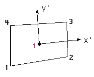
Gauss Points positions of the quadrature of Gauss-Legendre for Triangles and Quadrilaterals
This field is meaningless to lines, and should be set to 1
- 0 - the Natural Coordinates for the Gauss points will be the ones which are described below,
for Triangles and Tetrahedras they should be between 0.0 and 1.0, and for Quadrilaterals
and Hexahedras should be between -1.0 and 1.0.
For instance, the Natural Coordinates of three Gauss Points on Triangles will be:
data_loc= this option indicates whether the nodes are included inside the number of points over lines or not.- 1 - nodes are not included in the points count for lines, so points are placed
at a distance from the nodes
i / ( n_points + 1)withi = 1..n_pointsandn_points >= 1. - 2 - nodes are included in the points count for lines, so points are placed
at a distance from the nodes
( i - 1) / ( n_points - 1)withi = 1..n_pointsandn_points >= 2.
- 1 - nodes are not included in the points count for lines, so points are placed
at a distance from the nodes
desc_compdoes not matter, but it must be specified.
Old postprocess mesh format |
The old postprocess mesh format is still compatible with this version of GiD. The files containing the postprocess mesh (in the old file format) can be separated into two categories:
- 3D Data Files:
ProjectName.post.msh, or the oldProjectName.flavia.msh, for volume mesh information andProjectName.post.bon, or the oldProjectName.flavia.bon, for surface mesh information. - 2D Data Files:
ProjectName.post.dat, or the oldProjectName.flavia.datfor 2D mesh information.
Postprocessing data files are ASCII files and must be in a specific format, which is explained below. Each mesh information file can only handle one type of element.
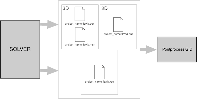
- ProjectName.flavia.msh:
The first file, which is named
ProjectName.flavia.msh, should contain the information relative to the 3D volume mesh. It contains the nodal coordinates of the 3D mesh, its nodal connectivities and the material of each element. The nodal coordinates must include those on the surface mesh. If no material is supplied, GiD takes the material number equal to zero. - ProjectName.flavia.bon:
The second file, which is named
ProjectName.flavia.bon, should contain the information about 3D surface sets. It can be used to represent boundary conditions of the volumetric mesh and additional surfaces (for instance, sheets, beams and shells). At least, all the mesh points supplied inProjectName.flavia.mshshould be present inProjectName.flavia.bonat the beginning of the file. - ProjectName.flavia.dat: This file contains information about 2D meshes. And only can be used if none of the two above are used. It should specify nodal coordinates of the meshes, its connectivities ( elements) and, if desired, its material number ( if not specified, GiD takes to be 0). The files are created and read in the order that corresponds with the natural way of solving a finite element problem: mesh, surface definition and conditions and finally, evaluation of the nodal results. The format of the read statements is normally free, i.e. it is necessary only to separate them by spaces. Thus, the users can modify the files with any format, leaving spaces between each field and can also write out the results with as many decimals as desired. In case of error, the program warns the user about the type of mistake found. GiD reads all the information directly from the pre-processing files in order to gain efficiency, whenever possible).
Old format - File ProjectName.flavia.msh |
Set 1: Header
The total number of lines in this set is 6. All of them are free lines for any use. This will be the case of the first five lines, which may have an information role, informing about the project name, current version, as well as extra comments that can seem useful to add. Although they can be skipped, they are kept as a particular option inside GiD (comment lines) and as an utility to comment some additional information, like the type of project, equations, conditions and others.
Note: It is advisable, as it occurs in different solver modules used by GiD, that the sixth line explains the contents of the seventh line.
Set 2: General mesh data
The total number of lines in this set is 1, composed by at least 3 integers, the 4th integer is optional:
n_3D_mesh_elements n_3D_mesh_points n_element_type [ last_node]
where:
n_3D_mesh_elements= number of mesh elements.n_3D_mesh_points= number of mesh points.n_element_type= type of elements.last_node= number of the last node and required if nodes are not between 1 andn_3D_mesh_points.
The third parameter is used by the program to recognize what kind of finite element is being used. To do this in a standard way, GiD considers the following finite element types:
- number 1 corresponds to a hexahedra with eight nodes.
- number 3 corresponds to a tetrahedra with four nodes.
Set 3: Free line for any use
The total number of lines in this set is 1, which is a free line for any use, though most modules inside GiD write here the word 'Coordinates' to point the meaning of the following lines.
Set 4: Coordinates
The total number of lines in this set is n_3D_mesh_points, one for each
nodal point, composed by 1 integer plus 3 reals numbers:
i x_coord[i] y_coord[i] z_coord[i]
where:
i= node number.x_coord[i]= x_coordinate of the node numberi.y_coord[i]= y_coordinate of the node numberi.z_coord[i]= z_coordinate of the node numberi.
All the points of the meshes of the domain have to appear in this file.
Set 5: Free line for any use
The total number of lines in this set is 1, which is a free line for any use. The same comments used for set number 3 are valid here, with the change of including the word 'Connectivities' instead of 'Coordinates'.
Set 6: Connectivities
The total number of lines in this set is n_3D_mesh_elements, composed by 1
integer plus n_nodes/element integers and 1 optional integer more:
j node[j][1] node[j][2] ... node[j][n_nodes/element]
mat[j]
where:
j= element number.node[j][1]= node number 1 for the element numberj.node[j][2]= node number 2 for the element numberj. ...node[j][n_nodes/element]= last node number for the element numberj.mat[j]= material index of the element numberj.
The nodal connections must follow some specifications, so, for each tetrahedral element with four nodes, the rule is that the first three nodes that form a triangular face must be so sorted in order to define a normal which points towards the semi space containing the fourth node.
The vector mat[j] holds
the material index of the element number j.
Old format - File ProjectName.flavia.bon |
The total number of lines in this set is 6. All of them are
free lines for any use. All the comments relative to the header of
ProjectName.flavia.msh remain
valid for the current file ProjectName.flavia.bon.
Note: It is advisable, as it occurs in different calculation modules included in GiD, that the sixth line explains the contents of the seventh line. Set 2: General boundary data
The total number of lines in this set is 1, composed by at least 3 integers, the 4th integer is optional:
n_bound_elements n_bound_points n_element_type [ last_node]
where:
n_bound_elements= number of boundary elements.n_bound_points= number of boundary points.n_element_type= type of elements.last_node= number of the last node and required if nodes are not between 1 andn_bound_points.
For the third parameter, GiD considers the following finite element types:
- number 7 corresponds to a triangle with three nodes.
- number 9 corresponds to a quadrilateral with four nodes.
- number 11 corresponds to a line with two nodes.
Set 3: Free line for any use The total number of lines in this set is 1, which is a free line for any use, though most modules inside GiD write here the word 'Coordinates' to point the meaning of the following lines.
Set 4: Coordinates
The total number of lines in this set is n_bound_points, one for each
nodal point, composed by 1 integer plus 3 reals:
i x_coord[i] y_coord[i] z_coord[i]
where:
i= node number.x_coord[i]= x_coordinate of the node numberi.y_coord[i]= y_coordinate of the node numberi.z_coord[i]= z_coordinate of the node numberi.
All the points of the domain have to appear in this file, what includes all the
mesh points introduced in ProjectName.flavia.msh at the beginning. Once all the
volumetric mesh had been introduced, it is possible to add surfaces that belong
to a boundary of the domain but do not belong to a volumetric mesh and by this
reason they will not appear in ProjectName.flavia.msh and only in
ProjectName.flavia.bon.
Set 5: Free line for any use The total number of lines in this set is 1, which is a free line for any use. The same comments used for set number 3 are valid here, with the change of including the word 'Connectivities' instead of 'Coordinates'.
Set 6: Connectivities
The total number of lines in this set is n_bound_elements, composed by 1
integer plus n_nodes/element integers and 2 optional integers more:
j node[j][1] node[j][2] ... node[j][n_nodes/element]
set[j]
where:
j= element number.node[j][1]= node number 1 for the element numberj.node[j][2]= node number 2 for the element numberj. ...node[j][n_nodes/element]= last node number for the element numberj.set[j]= number of set to which the element numberjbelongs.
The vector set[j] allows to distinguish groups of elements in different sets.
It applies, for instance, in the case of defining the different conditions
that the element fulfills.
Old format - File ProjectName.flavia.dat |
The total number of lines in this set is 6. All of them are free lines for any use. The first five lines, which may have an information role, informing about the project name, current version, as well as extra comments that can seem useful to add. Although they can be skipped, they are kept as a particular option inside GiD (comment lines) and as an utility to comment some additional information, like the type of project, equations, conditions and others.
Note: It is advisable, as it occurs in different solver modules used by GiD, that the sixth line explains the contents of the seventh line. Set 2: General mesh data
The total number of lines in this set is 1, composed by at least 3 integers, the 4th integer is optional:
n_2D_mesh_elements n_2D_mesh_points n_element_type [ last_node]
where:
n_2D_mesh_elements= number of 2D mesh elements.n_2D_mesh_points= number of 2D points.n_element_type= type of elements.last_node= number of the last node and required if nodes are not between 1 andn_2D_mesh_points.
The third parameter is used by the program to recognize what kind of finite element is being used. To do this GiD considers the number of nodes that the finite element type uses. So,
- number 2 corresponds to a line with two nodes.
- number 3 corresponds to a triangle with three nodes.
- number 4 corresponds to a quadrilateral with four nodes.
- number 6 corresponds to a triangle with six nodes.
- number 8 corresponds to a quadrilateral with eight nodes.
- number 9 corresponds to a quadrilateral with nine nodes.
Set 3: Free line for any use The total number of lines in this set is 1, which is a free line for any use, though most modules inside GiD write here the word 'Coordinates' to point the meaning of the following lines.
Set 4: Coordinates
The total number of lines in this set is n_2D_mesh_points, one for each
nodal point, composed by 1 integer plus 3 reals:
i x_coord[i] y_coord[i]
where:
i= node number.x_coord[i]= x_coordinate of the node numberi.y_coord[i]= y_coordinate of the node numberi.
All the points of the domain have to appear in this file, what includes all the
mesh points introduced in ProjectName.flavia.msh at the beginning. Once all the
volumetric mesh had been introduced, it is possible to add surfaces that belong
to a boundary of the domain but do not belong to a volumetric mesh and by this
reason they will not appear in ProjectName.flavia.msh and only in
ProjectName.flavia.bon.
Set 5: Free line for any use The total number of lines in this set is 1, which is a free line for any use. The same comments used for set number 3 are valid here, with the change of including the word 'Connectivities' instead of 'Coordinates'.
Set 6: Connectivities
The total number of lines in this set is n_2D_mesh_elements, composed by 1
integer plus n_nodes/element integers and 2 optional integers more:
j node[j][1] node[j][2] ... node[j][n_nodes/element]
set[j]
where:
j= element number.node[j][1]= node number 1 for the element numberj.node[j][2]= node number 2 for the element numberj. ...node[j][n_nodes/element]= last node number for the element numberj.set[j]= number of set to which the element numberjbelongs.
The vector set[j] allows to distinguish groups of elements in different sets.
It applies, for instance, in the case of defining the different conditions
that the element fulfills.
Note: The numeration of quadratic elements is linear and not hierarchical, i.e. nodes should be specified counterclockwise, without jumping internal nodes.
Go to the first, previous, next, last section, table of contents.
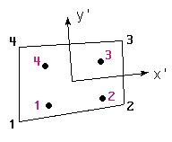 a=0.57735027
 a=0.77459667
 a=1/3
Internal coordinates:
 a=1/2
a=1/2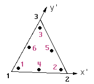 a=0.09157621 b=0.81684757