POSTPROCESSING RESULTS |
The possible results to be displayed can be grouped into five major categories:
- Scalar view results: Show Minimum & Maximum, Contour Fill, Contour Text Ranges, Contour Lines, Iso Surface and its configuration options.
- Vector view results: Mesh deformation, Display Vectors, Stream Lines (Particle Tracing)
- Line diagrams: Scalar line diagram and vector diagrams.
- Graph lines: XY plots.
- Animation: animation of the current result visualization.
The View Results menu and the View Results window are used to manage the visualization of the different type of results.
![]()
The View Results menu lets you select any type of result:
- Contour fill
- Contour ranges
- Contour lines
- Display vectors
- Show min/max
- Iso surfaces
- Stream lines
- Graphs
- Deformation
- Line diagrams
![]()
The View Results window manages the visualization of the following type of results:
- Contour fill
- Contour ranges ( if
Result Range Tables are present) - Contour lines
- Display vectors
- Show min/max
- Scalar and Vector line diagram ( if Linear elements are present)
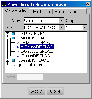
View Results Window
As the results are grouped into steps and analysis, GiD must know which analysis and step is
the currently selected for displaying results.
The Analysis menu of the View Results window is used to select the current analysis and step to be used for the rest of the results options. If some of the results view requires another analysis or step, the user will be asked for it.
Note: To stop viewing a result, the user can select No Result in this window or in the View results menu.
Contour Fill |
![]()
This option allows the visualization of colored zones, in which a variable, or a component, varies between two defined values. GiD can use as many colors as allowed by the graphical capabilities of the computer. When a high number of colors is used, the variation of these colors looks continuous, but the visualization becomes slower unless the Fast-Rotation option is used. A menu of the variables to be represented will be shown, from which the one to be displayed will be chosen, by using the default analysis and step selected.
Vectors will be unfolded into X, Y, and Z components and its module. Symmetric matrix values will be unfolded into Sxx component, Syy component, Szz component, Sxy component, Syz component and Sxz component of the original matrix and also into Si component, Sii component and Siii component in 3D problems or angular variation in 2D problems. Any of these components can be selected to be visualized.
When using results defined over gauss points, they are extrapolated to the nodes. So discontinuities can appear between adjacent elements. If the gauss points results cannot be extrapolated to the nodes, they are drawn as coloured spheres. The radius and detail level of these spheres can be configured too (see section Point and Line options).
Several configuration options can be accessed via the Options menu.
![]()
- Number Of Colors: Here the number of colors of the results color ramp can be specified.
- Width Intervals:
fixes the width of each color zone. For instance, if a
width intervalof 2 is set, each color will represent a zone where the results differ at the most in two units. - Set Limits: this option is used to tell the program which contour limits should use when there are no user defined limits: the absolute minimum and maximum of all sets or shown sets, for the actual step or for all steps.
- Define limits:
when choosing this option the
Contour Limitswindow appears (this option is also available in the postprocess toolbar). With this window the user can set the minimum/maximum value that Contour Fill should use. Outliers will be drawn with the color defined in theOut Min Color/Out Max Coloroption. - Reset Limit Values:
this option resets the values defined in the
Define limitsoption. - Reset All: this option sets all Contour Fill options by default.
- Max/Min Options:
Inside this group, several options for the minimum or maximum value can be defined:
- ResetValue: here the user can reset the maximum/minimum value, so that the default value is used.
- OutMaxColor / OutMinColor:
with this option the user can specify how the outliers values should be drawn:
Black,Max/Min Color,TransparentorMaterial. - Def. MaxColor / Def. MinColor: this option lets the user define the color for the minimum or maximum value for the color scale to start with.
- Color scale:
Specifies the properties of the color scale:
- Standard: the color scale will be the default: starting from blue (minimum) through green until red (maximum).
- Inverse Standard: the color scale will just be the inverse of the default: starting from red (minimum) through green until blue (maximum).
- Terrain Map: a physical-map like color ramp will be used.
- Black White: Black for Minimum and White for Maximum, the scale will be a grey ramp.
- Scale Ramp:
this option lets the user specify how should the ramp change from minimum color to the maximum color:
Tangent,ArcTangentorLinear. The default isArcTangent. - Scale Type:
tells GiD how the colors between the minimum color and the maximum color should change:
RGBorHSV.
- Color window: a window is poped up to let the user configure the colour scale of the contours easily
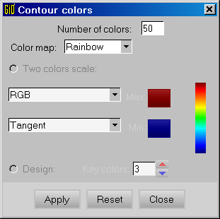
Contour Colours Window
Smooth Contour Fill |
![]()
This option displays a Contour fill, explained in the previous section, of a local smoothing of the results defined over gauss points.
With the Smoothing type option inside the menu Options->Contour
the user can choose between these types of local smoothing:
- Minimum value: as nodal results the minimum of the extrapolated gauss points results of the adjacent elements are used.
- Maximum value: as nodal results the maximum of the extrapolated gauss points results of the adjacent elements are used.
- Mean value: as nodal results the mean value of the extrapolated gauss points results of the adjacent elements are used.
Contour Ranges |
![]()
This is the same as the Contour Fill visualization type, but the coloured areas are
created following a 'Result range table' specified in the results file,
see section Result Range Table, and the name of these areas are also visualized as text labels.
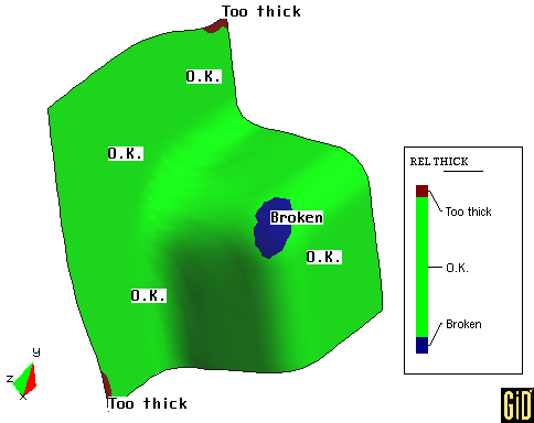
Contour ranges example
Contour Lines |
![]()
This display option is quite similar to contour fill (see section Contour Fill), but here, the isolines of a certain nodal variable are drawn. In this case, each color ties several points with the same value of the variable chosen.
Here the configurations options are almost the same than the ones for Contour Fill
(see section Contour Fill), with the only difference that the number given in the
Number of Colors option will be used as the number of lines for this contour lines representation.
Show Minimum and Maximum |
![]()
With this option the user can see the minimum and maximum of the chosen result.
Note: This minimum and maximum can be absolute, for all the meshes/sets/cuts, or relative (local) to the shown ones.
This can be selected from the top menu Options -> Contour -> Set Limits.
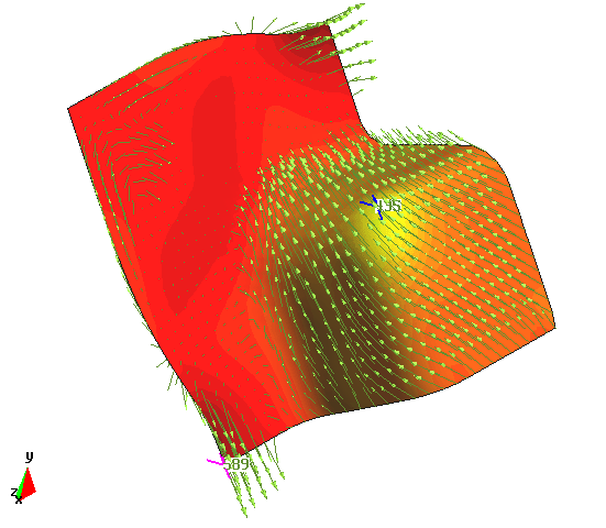
Display vectors |
![]()
This option displays a menu with results from vectors and matrices (where the principal values are previously evaluated by the program). A menu of variables to be represented will be shown, from which the one to be seen should be chosen, using the default analysis and step selected. Once a vector is chosen, the program will display the nodal vectors of the chosen result. The drawn vectors can be scaled interactively. The factor can be applied several times and every time it changes to the new input value.
The user can modify the colour of the vectors, which, by default, are drawn in green, so that all the vector are drawn with the same colour, or let the vectors colour vary according to the result module.
When drawing a matrix result, such as the stress tensor, only a single color representation of principal values is available: blue when negatives (also drawn as >--< representing compressions), and red when positives (also drawn as <--> representing tensions).
Vectors will be unfolded into X, Y, and Z components and its module. So only the X, Y or Z component can be drawn or the whole vector, which is represented by the module menu option. Symmetric matrices will be unfolded into Si component, Sii component, Siii component and 'All' components. Any of these components can be selected to be visualized. Si, Sii and Siii represent the eigen values & vectors of the matrix results which are calculated by GiD, and which are ordered according to the eigen value.
Several configuration options can be accessed via the Options menu.
![]()
Color Mode:
This option lets the user choose if vectors are drawn in one color (Mono Color) or in several colors (Colour Modules).
Number of Colors:
If the user uses Colour Modules to draw vectors, it is possible to choose the number of colors.
Offset: With this option, the user controls where the vector should be in relation of the node, ranging from 0, to tie the tail of the arrow to the node, to 1, to tie the tip of the arrow to the node.
Note: These options have no effect when viewing a matrix result.
Colour (mono): When vectors are drawn in (Mono Color) Color Mode, they are drawn
in green. The user can change this green colour selectiong this entry.
Detail: The level of detail can be adjusted to draw the vectors quicker or nicer. The different options are:
- Point: the arrow head will be drawn as a point. The style used to draw these point like arrow heads can be modified through the point options window described before, see section Point and Line options.
- Lines: the arrow head will be drawn as four lines.
- 2 Triangles: the arrow head will be drawn with 2 self intersecting triangles.
- 4 Triangles: the arrow head will be drawn as cones of 4 triangles.
- 8 Triangles: the arrow head will be drawn as cones of 8 triangles.
Note: This last option affects also matrix and local axes results.
Iso Surfaces |
![]()
Here a surface is drawn that ties a fixed value inside a volume mesh. A line is drawn for surface meshes. To create iso-surfaces there are several options:
- Exact: After choosing a result, or a result component, of the current analysis and step, the user can input several fixed values and then for each given value a iso-surface is drawn.
- Automatic: Similarly, after choosing a result, or a result component, the user is asked for the number of iso-surfaces to be created. GiD calculates the values between the Minimum and the Maximum (these not included).
- Automatic Width: After choosing a result, or result component, the user is asked for a width. This width is used to create as many iso-surfaces as needed between the Minimum and the Maximum (these included) values defined.
Several configuration options can be accessed via the Options menu.
![]()
- Display Style:
For Iso-Surfaces there is also a
Display Styleoption, like for Volumes/Surfaces/Cuts. The optionsAll Lines,Hidden Lines,Body,Body Linesare available. (see section Display Style) - Render:
The
renderoption for Iso-Surfaces renders that surfacesFlatorNormal. (see section Display Style) - Transparency:
The Iso-Surfaces can be set to
TransparentorOpaque. (see section Display Style) - Convert to cuts:
Another interesting option is
Convert To Cuts. With this options all the Iso-Surfaces drawn will be turn into cuts, so that they can be saved, read, and used to drawn results over them.
Stream Lines |
![]()
With this option the user can display a stream line, or, in fluid dynamics, a particle tracing, in a vector field. After choosing a vector result, using the default analysis and step selected, the program asks the user for a point to start with the plotting of the stream line. This point can be given in several ways:
-
just clicking on the screen: the point will be the intersection between the line orthogonal
to the screen and the plane parallel to the screen and containing the
Rotation center, - joining a node: the selected node will be used as a start point,
- select nodes: here several nodes can be selected to start with,
- along line: with this option the user can define a segment, along which several start points will be chosen. The number of points will also be asked for, including the ends of the segment. In case of just one point start, this will be the center of the segment.
- in a quad: the user can enter here four lines that define a quadrilateral area which will be used to create a N x M matrix of points. These points will be the start for the stream lines. When giving N x M, N lies on the first and third line, and M on the second and fourth. So, points ( 0, 0..N), ( M, 0..N), ( 0..M, 0) and ( 0..M, N) will lie just on the lines. But in case of N=1 or M=1, this will be the center of the line, and if N = 1 and M = 1, this will be the center of the Quad.
- intersectset the point will be the intersection between the line orthogonal to the screen and the current viewed sets nearest the viewpoint.
When viewing Stream Lines, labels can be drawn to show the times at start and end points
of the stream line.
Stream lines can also be deleted, and its, by default, green colour can be changed too.
Following options can be chosen for Stream Lines:
![]()
Color: the colour of the stream lines.
Delete: this option lets the user select stream lines to be deleted.
Label: this option lets the user select the kind of label:
None: no labels are drawn.0_End: labels are drawn with the following convention: 0 at the start of the stream line and the total time taken for the particle to travel at the end.Ini_End: labels are drawn with the following convention: 0 at the chosen point, and- time beforeat the begin of the stream line andtime afterat the end.
Size & detail: here the user can adjust the wise, width, and detail of the stream lines using a window ( see section Point and Line options).
Line diagrams |
![]()
This result visualization option is only active when line elements are used in the mesh, and only will be represented over these line elements. When using this result visualization option, graph-style lines will be drawn over the line elements.
When drawing a Scalar Diagrams the graph-style lines are drawn on a plane parallel to the screen ( with its normal vector pointing to the user) when this result view is selected. The positive 'axis' will be the vector resulting of the cross product between this normal vector and the one that the line defines.
When drawing a Vector Diagrams the graph-style lines are drawn on a plane that withholds the result vector and the one that the line defines. The graph-style line represent the module of this vector. The positive 'axis' is also defined by the result vector. As modules are positive, to allow negative values, the input format for vector results allows the introduction of a fourth component: the signed vector module (see section Postprocess results format: ProjectName.post.res, ProjectName.flavia.res).
There is a Show Elevations option only accessible through the Right buttons menu
under 'Results / LineDiagram / Options'. Elevations are lines that connect the nodes
and the gauss points of the line element and the graph style line that represents the result.
The options are:
- None: to switch the elevations off,
- Nodes only: to draw the elevation lines only on the nodes,
- Whole line: to draw the elevation lines along the whole line, using nodes and gauss points,
- Filled line: to draw orange filled elevations,
- Contour filled line: the colours used to draw the filled elevations will be the same as of a contour fill done along the line.
Legends |
![]()
Legends appear when Contours visualization, iso-surfaces or color vector visualization are used:
- Show: legends can be switched on and of.
- Opaque: legends can be transparent, showing the result visualization behind them, or not.
- Show title: with this option the result name of the current visualization appears on the top of the legend.
- Outside: activating this option, the legend is shown on a separate window, thus freeing precious graphical surface on GiD's windows.
- Automatic comments: if this option is activated, information about the type of analysis, the actual step and the kind of result, is added at the bottom of the screen see section Automatic comments.
Graphs |
![]()
![]()
Graph Lines description |
Here the user can draw graphs in order to have a closer look to the results. Several graphs types are available: point evolution against time, result 1 vs. result 2 over points and result along a boundary line. The user can also save or read a Graph (see section Files menu). The format of the file will be described later. (see section Graph Lines File Format)
Under the Graphs option of the View Results menu there are the following options:
Show: here the user can switch between the graphs view and the post-processing view.ClearGraphs: to reset all the graphs and do a new start.Point Evolution: this graph shows the evolution of a result on a point along all the steps in the current analysis.Point Graph: after choosing a point or points, the user can contrast a result against another.Border Graph: after selecting a border, the user can see how the results varies along this boundary. You can also use theBorder Graphwindow (Windowsmenu) to configure this type of graphs.
The user can also view the labels of the points of the graphs, not only the Graph points number, but also theirs X and Y values. If some points of the Graphs are labeled, when turning into the normal results view, the labels also appear on the results view.
Graph Lines options |
![]()
Grids: here the user tells whether to drawn grids or not.Current Style: the user can choose how the new graphs should look like. The possible styles areDot,LineandDot-Line.Change Style Graph: the user can change the style of the selected graph.Change Colour Graph: herewith the colour of the selected graph can be changed.Change Line Width Graph: the width of the graph lines can be changed too.Change Line Pattern Graph: this option is useful to switch between different line patters for a b/w printer.Change Point Size Graph: also the point size can be changed for theDotandDot-Linestyles.Change Style Graph: the user can change the style of the selected graph.Change Title Graph: the user can change the title of the selected graph.Title: the user can change the title, its position or reset its value.X_Axis: here the user can set min and max values and divisions for the X axis, reset them, and change its Label.Y_Axis: here the user can set min and max values and divisions for the Y axis, reset them, and change its Label.
Graph Lines File Format |
The Graph file that GiD uses is an standard ASCII file. Every line of the file
is a point of the Graph with X and Y coordinates separated by a space.
Comment lines are also allowed and should begin with a '#'. The title of the Graph and
the labels for the X and Y axis can also be configured. If a comment line contains
the Keyword 'Graf:' the string between quotes that follows this keyword will be used as
title of the graf. The string between quotes that follows the Keyword 'X:' will be used as
label for the X axis. The same is also true for the Y axis, but for the Keyword 'Y:'.
Here an example:
        # Graf: "Nodes 26, 27, 28, ... 52 Graf."
        #
        # X: "Szz-Nodal_Streess" Y: "Sxz-Nodal_Stress"
        -3055.444 1672.365
        -2837.013 5892.115
        -2371.195 666.9543
        -2030.643 3390.457
        -1588.883 -4042.649
        -1011.5 1236.958
        # End
Result surface |
This option uses a result component, or a scalar value, and draws a 3D surface above the mesh following the normals of this mesh. It can be seen as an extrusion of the mesh along their normals with the result as factor. Like the beam diagrams but with surfaces.
With the Show elevations option inside the menu Options->Result Surface
the user can choose how the elevations ( lines or faces that connect the Result Surface with the underlaying mesh) are drawn:
- None: The mesh and its result surface are drawn separately, without interconnecting lines or faces.
- Extruded nodes: lines are drawn between the original nodes of the mesh and the extruded ones, the ones of the result surface.
- Extruded edges: faces are drawn between the original edges (of the elements) of the mesh and the extruded ones, the ones of the result surface.
- Contour fill: with this option the user can switch on and off the contour fill representation of the result used to create the 3D surface.
Deform Mesh |
![]()
Volumes, surfaces and cuts can be deformed according to a nodal vector and a factor. When doing so
all the results are drawn on the deformed volumes, surfaces and cuts. This is called in
GiD: Main Geometry. Thus, when the Main Geometry is deformed, results are
also drawn deformed; and when Main geometry is in its original state, results are
also drawn in its original state.
View results window allows to do this.
![]()
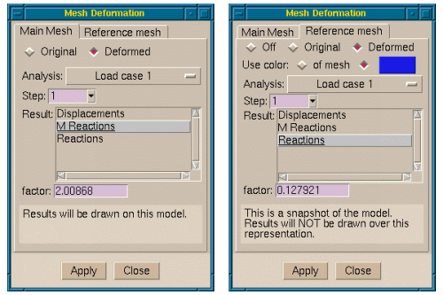
Deformation Window
On the upper part of this window, the user can choose between the Original state of the
Main Geometry and the Deformed state, for which a nodal vectorial result, and
an analysis and step, must be selected and a factor entered.
There is also a so-called Reference Geometry option. This allows to visualize volumes, surfaces or cuts like Main Geometry but NO results can be displayed over these volumes, surfaces or cuts.
It is merely provided as a reference, to contrast several deformation or changes of the original
geometry. Remember that the current Mesh Display Style will be used for the
Reference Geometry and it can be only changed when redoing it.
On the lower part of the Deform Mesh window, this Reference Geometry
can be configured. The user can choose between:
Off, so this reference visualization is not displayed.
Original, if Main Geometry is deformed and the user wants to compare it
with its original state without loosing a results representation.
Deformation, where,
after providing an analysis, step, result and factor, the user can use it
to contrast two deformation states, or a deformed state and an original geometry.
Color, the colour of the reference meshes can be the same as the original meshes,
or can be specified here.
Do Cuts |
![]()
Here the user can cut and divide volumes, surfaces and cuts. A cut of a volume mesh results into a cut plane. The cut is done for all the meshes, despite that some of them are switched off. When cutting surfaces, a line set will be created. Here only those surfaces that are switched on are cut.
Another feature is that a cut can be deformed, if meshes are also told to do so (see section Deform Mesh). A cut of a deformed mesh, when changing to the original shape, will be deformed accordingly.
When dividing volumes/surfaces only those elements of the volumes/surfaces switched on that lie on one side of a specified plane will be used to create another volume/surface.
- Cut Plane:
the user specifies a plane which cuts the volumes/surfaces. Several options can be used to enter
this plane. With
Two Points( the default), the plane is defined by the corresponding line and the orthogonal direction to the screen. WithThree Points, the plane is defined by this three points. When choosing the points, the nodes of the mesh can also be used. All the volume meshes are cut, whether they are drawn or not. - Divide Volume Sets:
the user specifies a plane which is used to divide the meshes. Several options can be used to enter
this plane. With
Two Points( the default), the plane is defined by the corresponding line and the orthogonal direction to the screen. WithThree Points, the plane is defined by these three points. When choosing the points, the nodes of the mesh can also be used. After defining the plane, the user should choose which section of the mesh should be saved by select the side of the plane to use. Only those elements that lie entirely on this side are selected. Only those volume meshes that are shown are divided. - Divide Surface Sets:
the user specifies a plane which is used to divide the sets. Several options can be used to enter
this plane. With
Two Points(the default), the plane is defined by the corresponding line and the orthogonal direction to the screen. WithThree Points, the plane is defined by these three points. When choosing the points, the nodes of the mesh can also be used. After defining the plane, the user should choose which section of the mesh should be saved by select the side of the plane to use. Only those elements that lie entirely on this side are selected. Only those surface meshes that are shown are divided. When doing a division, clicking with the right button mouse, inside the Contextual menu, there are several useful options:- exact: to do a exact division, i.e. elements are cut to create the division.
- parallel planes: the remaining elements will be ones between two parallel planes,
a
distancecan also be entered, after choosing this option from the same contextual menu
- Divide lines: the user specifies a plane which is used to get the lines at one side of this plane
- Succession:
This option is an enhancement of
Cut Plane. Here the user specifies an axis that will be used to create cut planes orthogonal to this axis. The number of planes is also asked for. - Cut Wire: Here the user can define a 'wire' tied to the edges of the elements of the volumes/surfaces. So when the volumes/surfaces are deformed, the wire is deformed too. And vice versa, if a wire is defined while the volumes/surfaces are deformed, when turning them into its original shape, the cut-wire is "undeformed" with them.
- Cut Spheres: Here the user can define a sphere which will be used to cut the volume and surface meshes, resulting in triangle or line cut meshes respectivelly.
- Convert cuts to surface sets: With this options cuts can be converted to surface sets so they can be saved, or cut again.
Cuts can also be read and write from/to a file. The information stored into the file from a 'Cut Plane'
is the plane equation that defines the plane ( Ax + By + Cz + D = 0), so it can be used with several models.
The information stored into the file from a 'Cut Wire' is the points list of the cut-wire, i.e. the
interseccion between the wire and the edges of the meshes/sets.
These files are standard ASCII files. A line of a 'Cut Plane' archive contains the four coefficients
of the cut defining plane separated by spaces. A line of a 'Cut Wire' archive contains the three
coordinates of a point of the wire. Comment lines are allowed and should begin with a '#'.
An example of a 'Cut Plane' archive where three planes were written:
        # planes created of a 'cut succession'
        -10.82439 0.5740206 0 51.62557
        -10.82439 0.5740206 0 12.45994
        -10.82439 0.5740206 0 -26.70569
An example of a 'Cut Wire' archive:
        -2.444425 3.883427 2.487002
        2.130787 2.762815 3.885021
        0.8411534 4.458836 3.215301
        4.270067 3.795048 2.037187
        5.66561 3.414776 0.8219391
        2.945865 3.600701 3.29012
        0.4487007 3.764661 3.574121
Animation |
![]()
With this window a little bit of automatization has been done to create animations inside GiD. Nowadays, almost all the results visualization are animated. Only stream-lines are not automatized along all the steps of the current analysis.
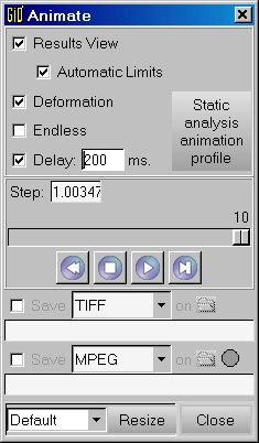
Animation Window
This window lets the user create an animation of the current Results View, where
the limits can be fixed along the animation with Automatic Limits, and/or of
the Deformation of the meshes.
On the right of the Step: label, the step value is shown. On the slide bar, the step
number is shown.
The four buttons under the slide bar are autoexplicative, they should 'Rewind', 'Stop', 'Play' and 'Step' the animation. Also clicking on the slide bar the animation can be stepped down or up. The green led will change to red when an animation is begin stored on a file, after pressing the 'Play' button. This led will change back to green when the animation is finished, or the 'Stop' button is pressed.
Options are:
Automatic Limits: here GiD searches for the minimum and maximum values of the results along all the steps of the analysis and uses them to draw the results view through all the steps.Endless: to do the animation forever.Delay: here the user can specify a delay time between steps in milliseconds.Save TIFF/GIFs on: with this option the user can save snapshots, in TIFF or GIF format, of each step, when the 'Play' button is pushed. Here the filename given will be used as a prefix to create the TIFF/GIFs, for instance, if the user writesMyAnimation, TIFF/GIF files will be created with namesMyAnimation-01.tif/MyAnimation-01.gif,MyAnimation-02.tif/MyAnimation-02.gif, and so on.Save MPEG/AVI True Color/AVI 15bpp/GIF on: giving here a filename, a MPEG/AVI/GIF file will be created when 'Play' button is pushed.
Note: To avoid problems when trying to view an MPEG format animation in Microsoft Windows, it is strongly recommended to use the Default menu to select a 'standard' size and press the Resize button. The graphical window will change to this 'standard' size. After finishing the animation, just selecting Default on the menu and pressing the Resize button, the previous size will be restored.Static analysis animation profile: if the project has only one step, it's possible to simulate an animation by generating intermediate steps. Use this option to automatically generate several frames, following a lineal, cosine, triangular or sinusoidal interpolation between the normal state and the deformed state.
Automatic comments |
![]()
While displaying results, comments can be automatically generated by switching on
the Automatic checkbox in the Comments window, which appears selecting
Utilities->Graphical->Comments.
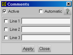
If this option is selected and the comment lines are empty, the program will create its own automatic comments, like these ones:
Load Analysis, step 3
Display Vectors of Displacements, |Displacements| factor 68095.4.
Deformation ( x127.348): Displacements of Load Analysis 2, step 8.
in bold, the fields which will change when the visualization changes.
The user can also create its own automatic comments, just filling the comment lines. To tell the program where the result name, analysis name, etc., should be placed, following fields can be used:
- %an: for analysis name of the current visualized result
- %sv: for step value of the current visualized result
- %vt: for result visualization type of the current visualized result
- %vf: for vectors factor used in the current visualized result ( if any)
- %rn: for result name of the current visualized result
- %cn: for component name of the current visualized result
- %da: for analysis name of the current deformation ( if any)
- %ds: for step value of the current deformation ( if any)
- %dr: for result name of the current deformation ( if any)
- %df: for factor of the current deformation ( if any)
GiD will substitute the fields by the values of the current visualization. Fields which cannot be fulfilled will be empty.
Several results |
![]()
With this window, which appears under Windows->Several Results, the user can select
whether to view the results one by one, as usual, or to view some results visualization types
at once, for instance a contour fill of pressure and velocity vectors at the same time.
From this window the user can also delete not desired results visualization.
After selecting the desired behaviour, the user should press the Apply button
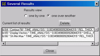
Several results window
Example showing contour fill, vectors and the minimum and maximum visualization types
Go to the first, previous, next, last section, table of contents.